Welcome to som-pbc’s documentation!

som-pbc

Authors: Alex Müller

This package contains a simple self-organizing map implementation in Python with periodic boundary conditions.

Self-organizing maps are also called Kohonen maps and were invented by Teuvo Kohonen.[1] They are an unsupervised machine learning technique to efficiently create spatially organized internal representations of various types of data. For example, SOMs are well-suited for the visualization of high-dimensional data.

This is a simple implementation of SOMs in Python. This SOM has periodic boundary conditions and therefore can be imagined as a “donut”. The implementation uses numpy, scipy, scikit-learn and matplotlib.

The project’s GitHub page can be found here: http://github.com/alexarnimueller/som

som-pbc README

A simple self-organizing map implementation in Python with periodic boundary conditions.

Self-organizing maps are also called Kohonen maps and were invented by Teuvo Kohonen.[1] They are an unsupervised machine learning technique to efficiently create spatially organized internal representations of various types of data. For example, SOMs are well-suited for the visualization of high-dimensional data.

This is a simple implementation of SOMs in Python. This SOM has periodic boundary conditions and therefore can be imagined as a “donut”. The implementation uses numpy, scipy, scikit-learn and matplotlib.

Installation

som-pbc can be installed from pypi using pip:

pip install som-pbc

To upgrade som-pbc to the latest version, run:

pip install --upgrade som-pbc

Usage

Then you can import and use the SOM class as follows:

import numpy as np
from som import SOM

# generate some random data with 36 features
data1 = np.random.normal(loc=-.25, scale=0.5, size=(500, 36))
data2 = np.random.normal(loc=.25, scale=0.5, size=(500, 36))
data = np.vstack((data1, data2))

som = SOM(10, 10)  # initialize a 10 by 10 SOM
som.fit(data, 10000, save_e=True, interval=100)  # fit the SOM for 10000 epochs, save the error every 100 steps
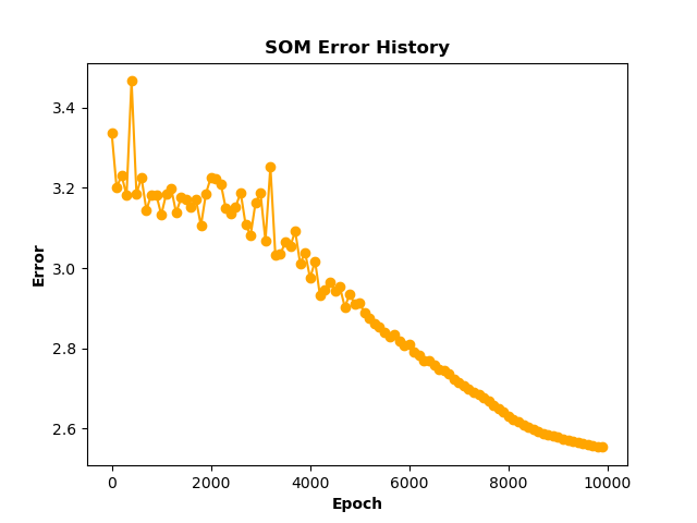
som.plot_error_history(filename='images/som_error.png')  # plot the training error history

targets = np.array(500 * [0] + 500 * [1])  # create some dummy target values

# now visualize the learned representation with the class labels
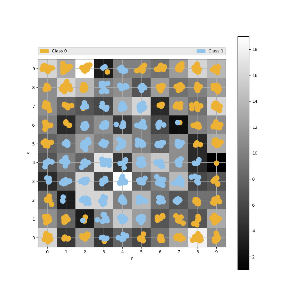
som.plot_point_map(data, targets, ['Class 0', 'Class 1'], filename='images/som.png')
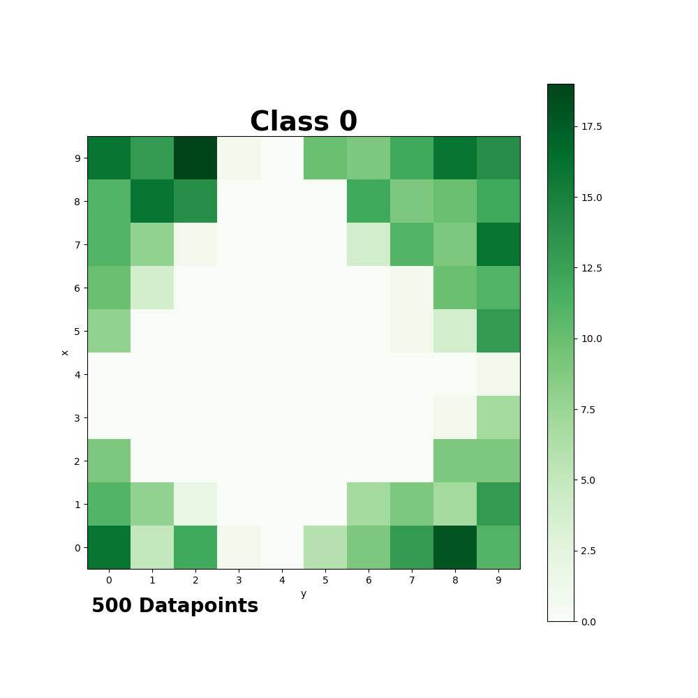
som.plot_class_density(data, targets, t=0, name='Class 0', colormap='Greens', filename='images/class_0.png')
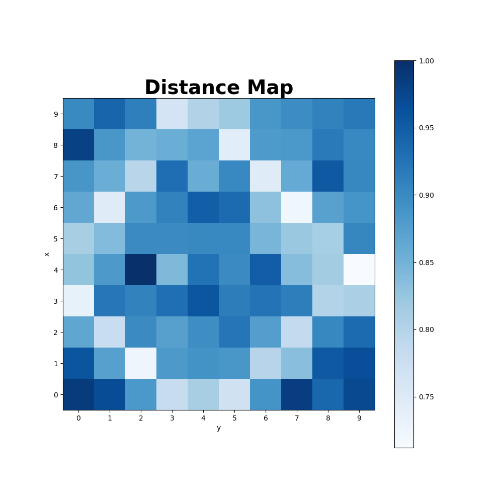
som.plot_distance_map(colormap='Blues', filename='images/distance_map.png')  # plot the distance map after training

# predicting the class of a new, unknown datapoint
datapoint = np.random.normal(loc=.25, scale=0.5, size=(1, 36))
print("Labels of neighboring datapoints: ", som.get_neighbors(datapoint, data, targets, d=0))

# transform data into the SOM space
newdata = np.random.normal(loc=.25, scale=0.5, size=(10, 36))
transformed = som.transform(newdata)
print("Old shape of the data:", newdata.shape)
print("New shape of the data:", transformed.shape)

Training Error:

Point Map:

Class Density:

Distance Map:

The same way you can handle your own data.

Methods / Functions

The SOM class has the following methods:

initialize(data, how='pca'): initialize the SOM, either via Eigenvalues (pca) or randomly (random)
winner(vector): compute the winner neuron closest to a given data point in vector (Euclidean distance)
cycle(vector): perform one iteration in adapting the SOM towards the chosen data point in vector
fit(data, epochs=0, save_e=False, interval=1000, decay='hill'): train the SOM on the given data for several epochs
transform(data): transform given data in to the SOM space
distance_map(metric='euclidean'): get a map of every neuron and its distances to all neighbors based on the neuron weights
winner_map(data): get the number of times, a certain neuron in the trained SOM is winner for the given data
winner_neurons(data): for every data point, get the winner neuron coordinates
som_error(data): calculates the overall error as the average difference between the winning neurons and the data
get_neighbors(datapoint, data, labels, d=0): get the labels of all data examples that are d neurons away from datapoint on the map
save(filename): save the whole SOM instance into a pickle file
load(filename): load a SOM instance from a pickle file
plot_point_map(data, targets, targetnames, filename=None, colors=None, markers=None, density=True): visualize the som with all data as points around the neurons
plot_density_map(data, filename=None, internal=False): visualize the data density in different areas of the SOM.
plot_class_density(data, targets, t, name, colormap='Oranges', filename=None): plot a density map only for the given class
plot_distance_map(colormap='Oranges', filename=None): visualize the disance of the neurons in the trained SOM
plot_error_history(color='orange', filename=None): visualize the training error history after training (fit with save_e=True)

References:

[1] Kohonen, T. Self-Organized Formation of Topologically Correct Feature Maps. Biol. Cybern. 1982, 43 (1), 59–69.

This work was partially inspired by ramalina’s som implementation and JustGlowing’s minisom.

Documentation:

Documentation for som-pbc is hosted on readthedocs.io.

Documentation for the som module

class som.SOM(x: int, y: int, alpha_start: float = 0.6, sigma_start: Optional[float] = None, seed: Optional[int] = None)

Class implementing a self-organizing map with periodic boundary conditions. It has the following methods:

cycle(vector: ndarray, verbose: bool = True)

Perform one iteration in adapting the SOM towards a chosen data point

Parameters

vector (np.ndarray) – current data point
verbose (bool) – verbosity control

distance_map(metric: str = 'euclidean')

Get the distance map of the neuron weights. Every cell is the normalised average of all distances between the neuron and all other neurons.

Parameters: metric (str) – distance metric to be used (see scipy.spatial.distance.cdist)
Returns: normalized sum of distances for every neuron to its neighbors, stored in SOM.distmap

fit(data: ndarray, epochs: int = 0, save_e: bool = False, interval: int = 1000, decay: str = 'hill', verbose: bool = True)

Train the SOM on the given data for several iterations

Parameters

data (np.ndarray) – data to train on
epochs (int, optional) – number of iterations to train; if 0, epochs=len(data) and every data point is used once
save_e (bool, optional) – whether to save the error history
interval (int, optional) – interval of epochs to use for saving training errors
decay (str, optional) – type of decay for alpha and sigma. Choose from ‘hill’ (Hill function) and ‘linear’, with ‘hill’ having the form y = 1 / (1 + (x / 0.5) **4)
verbose (bool) – verbosity control

get_neighbors(datapoint: ndarray, data: ndarray, labels: ndarray, d: int = 0) → ndarray

return the labels of the neighboring data instances at distance d for a given data point of interest

Parameters

datapoint (np.ndarray) – descriptor vector of the data point of interest to check for neighbors
data (np.ndarray) – reference data to compare datapoint to
labels (np.ndarray) – array of labels describing the target classes for every data point in data
d (int) – length of Manhattan distance to explore the neighborhood (0: same neuron as data point)

Returns

found neighbors (labels)

Return type

np.ndarray

initialize(data: ndarray, how: str = 'pca')

Initialize the SOM neurons

Parameters

data (numpy.ndarray) – data to use for initialization
how (str) – how to initialize the map, available: pca (via 4 first eigenvalues) or random (via random values normally distributed in the shape of data)

Returns

initialized map in SOM.map

load(filename: str)

Load a SOM instance from a pickle file.

Parameters: filename (str) – filename (best to end with .p)
Returns: updated instance with data from filename

plot_class_density(data: ndarray, targets: Union[list, ndarray], t: int = 1, name: str = 'actives', colormap: str = 'gray', example_dict: Optional[dict] = None, filename: Optional[str] = None)

Plot a density map only for the given class

Parameters

data (np.ndarray) – data to visualize the SOM density (number of times a neuron was winner)
targets (list, np.ndarray) – array of target classes (0 to len(targetnames)) corresponding to data
t (int) – target class to plot the density map for
name (str) – target name corresponding to target given in t
colormap (str) – colormap to use, select from matplolib sequential colormaps
example_dict (dict) – dictionary containing names of examples as keys and corresponding descriptor values as values. These examples will be mapped onto the density map and marked
filename (str) – optional, if given, the plot is saved to this location

Returns